GitHub Repo

I. Introduction

In this project, we look to provide a parallel solution to the problem of visual object detection presented in the original paper by Paul Viola and Michael Jones [1]. The original paper outlines a proposed algorithm as a solution for real-time face detection. We look to take this algorithm and port much of the functionality to a GPU. The areas of the original algorithm that we will be focusing on include the construction of Integral Images and parts of the AdaBoosting process. When computing the integral images, it is necessary to iterate through every pixel of every image in the dataset. Each pixel location includes the current row-sum for the given row, as well as the current column sum among the previous rows. This computation is run over several thousands of images, each of size 24x24 pixels. With the number of iterations of this process reaching several million, the process of integral image computation makes a good candidate for parallel execution. As we break down the learning algorithm proposed by Viola and Jones [1], we start to observe several iterative, independent routines that could also be parallelized. This paper focuses on two similar routines: training weak classifiers and computing classification errors. Both processes involve applying all features to all data samples and are two of the largest computational burdens of the entire algorithm. Since we have over 100,000 features and several thousand images, applying each feature to every image takes billions of operations. Feature applications to images are also independent of each other, making these processes ideal candidates for parallelization. By porting these operations to a GPU, we attempt to reduce these bottlenecks and decrease the computational time of each training iteration.

II. CPU Implementation and Algorithm

We will be briefly discussing the CPU implementation of the algorithm for completeness, as well as a means to display the transition from sequential code to parallel execution. The CPU implementation is almost directly taken from the original paper [1]. We will only be discussing the relevant sections of the code that will later be ported to the GPU.

Features

Before we start reviewing the implementation details, it is important to define some of the structures we will be working with throughout this project. This algorithm uses simple rectangular features that are applied to images in order to obtain a response value as a metric for classifying a subregion of an image. These simple rectangular features (see Figure 1) consist of rectangular sections that are to be summed over the input images. The difference between the sum of the sections within a feature is the response value for that feature for the given image. We use these features and their response values to classify whether or not a subregion of an image contains a face. This response value threshold identifying whether or not a face exists in a subregion is one of the metrics that is learned during the AdaBoosting phase. We will revisit this topic later on.

Integral Images

Integral images, or summed area tables, are used in this project to allow feature application to be reduced down to a few operations. Instead of having to perform the sum for each section of each feature on every image, we can simply take a few values from the integral image intermediate and calculate the sum in an efficient manner. The CPU implementation for integral images is fairly straight forward (see Figure 2). In order to calculate the integral image value at a given pixel, we must sum up all of the values to the left of the pixel in the same row and add this running sum to the current pixel value in the image. After this, the same is done for all of the pixels above the current coordinate in the same column. Here is the sequential integral image pseudo-code:

On the CPU, this process takes the form of two nested for-loops iterating through the rows and columns of an image. This process is done for every image that is in our dataset, thus producing three nested loops and millions of operations for the entire dataset. It is these three nested loops we look to parallelize.

Training

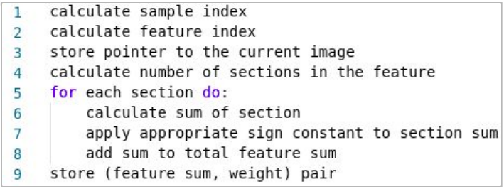
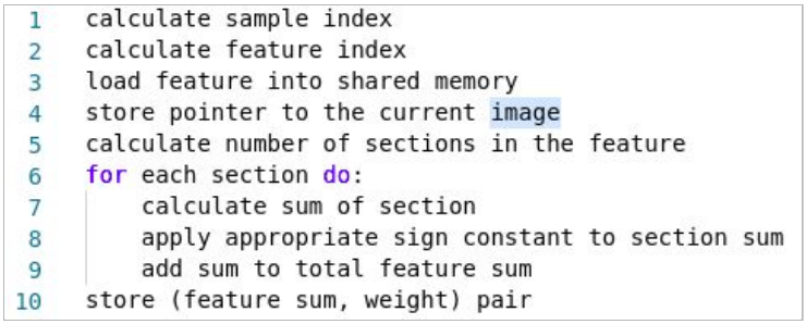
As previously stated, the focus of this paper will include only a subset of the learning algorithm involved in the original Face Detection paper [1]. For a more general overview of the learning process used by Viola and Jones, I recommend taking a look at their work. The first subsection we will be taking a look at is that of training weak classifiers. A weak classifier in this context includes a feature, a parity, and a threshold. The parity and the threshold values will be used later in the classification stage and can be ignored for now. This stage works with the response value obtained from applying the feature of the weak classifier to each image in our dataset. Since we do not know a priori which features will give us the best results for classifying faces in images, we must loop through our entire feature bank and apply every feature to every image. The application of each feature involves taking each section of the feature being applied and calculating the sum of the region of the image where sections overlap. In our implementation, we sum all sections of a feature after applying a sign constant to each section sum. The sign constant for the dark and light sections are -1 and 1, respectively. This is equivalent to subtracting the sum of the dark sections from the sum of the light sections and allows us to use the same addition operation for all sections. Here is the sequential training in pseudo-code:

The goal of this stage is to produce application response values for each weak classifier on each image. The later stages of learning use this information to produce an optimal parity and threshold for each weak classifier that will produce the best classification results possible and minimize the number of misclassified samples for the classifiers.

Classification

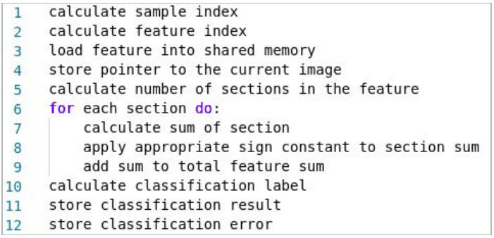
The classification stage is almost identical to that of the training stage. Every feature is applied to every image, just as in training; however, instead of storing the resulting response values from the application process, the parity and the threshold are used to make a binary classification for each image specifying whether or not the weak classifier has detected a face. This classification label is then compared to the actual label of the image. The errors, as well as the classification labels, for all combinations of features and images are recorded. Here is the sequential classification pseudo-code:

In order to calculate the classification label, the following equation is used:

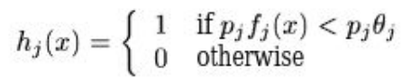
Here, h_j represents the weak classifier, x represents a 24x24 pixel image, f_j is the feature for the weak classifier, p_j is the parity, and Θ_j is the threshold.

III. GPU Implementation

In this section, we will propose parallel solutions to the above implementations for use on a GPU. Most of the optimizations we shall look to implement include an optimized use of the memory hierarchy, as well as trade-offs between simpler kernel computations and multiple kernel launches. As we will also depict in the results of this project, we attempted to compare the differences of using pointers on the GPU as opposed to creating deep copies of data and allocating pitched arrays on the device for our more complex structures. There was a large difference in computation time between these two methods, with pointer allocating taking much more time relatively. The examples we display throughout this paper will be using pitched data allocation.

Integral Images

The approach for calculating integral images on a GPU was inspired by Bilgic et al. [4]. Their work highlights an approach for efficient integral image computation on a GPU. Their approach is mainly directed at the scenario where the images being summed are large. This would normally be the case for the latter part of this face detection algorithm, where we would be identifying faces in large images. For the section we are highlighting in this report, all the images used are subregions of 24x24 pixels. Since these images can fit inside a block, we have adapted the approach to follow the Kogge-Stone Parallel Scan Algorithm [2]. This is an inclusive scan algorithm that works best when the rows being summed fit inside a block. This method also helps to reduce divergence in the warps of a block. For our implementation, each block is responsible for an image and each thread in a block represents a pixel in the integral image. The first step is to calculate an intermediate representation of the integral image by summing over every row in each image following the parallel scan algorithm. Here is the initial scan kernel pseudo-code:

The next step in the pipeline is to take the transpose of the images in order to utilize the same scan kernel to compute the column-wise sum of the images. The transposition itself is fairly simple and can be found in the work by Bilgic et al. [4]. To enhance the initial implementation of the scan kernel and to reduce the bottle-neck of I/O operations, we use shared memory to store the images for each block. Each thread in a block loads the pixel value it is responsible for. Then all threads synchronize and the scanning operation continues within shared memory. This reduces the amount of global memory accesses each thread performs on average. Here is the enhanced scan kernel pseudo-code:

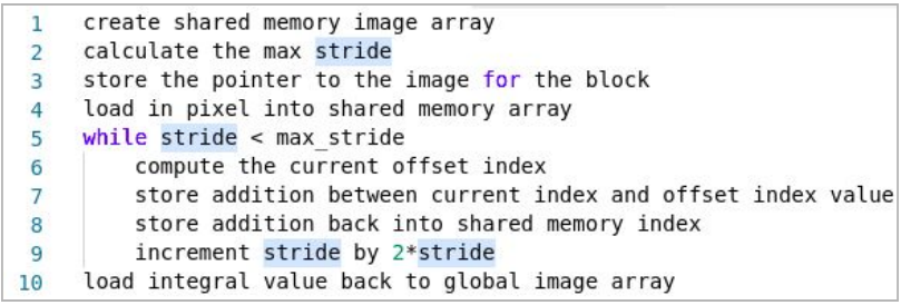
Since the summation happens in place, we need to synchronize after storing the sum in a register before we write the changes back to shared memory. In order to remove this dependency, we can implement double buffering. If we create a copy of the image in shared memory, we can keep pointers to a source and destination buffer. On each iteration, we read from the source buffer and write to the destination buffer without the need to synchronize. Then we swap the buffer pointers and continue on with the next iteration. Here is the enhanced scan kernel pseudo-code with double buffering:

Training

The approach to porting the training process to the GPU is mainly focused on how the kernel is launched and how much computation each thread performs. Our implementation holds each thread responsible for computing the application of a feature to an image. In order to launch the kernel under this approach, we use the max block size of 1024 threads and launch a sufficient amount of blocks so that we have enough threads to perform the application between each feature and image. The next task is to calculate the sample and feature index for each thread. Since we just launch enough threads to cover the combinations of features and images, we have to perform some computation to map the thread and block indexes to our sample and feature indexes:

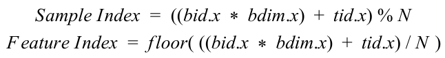
Here bid.x is our block index, bdim.x is the block dimension, tid.x is the thread index, and N is our total number of samples. The implementation itself is very similar to the CPU version. Here is the parallel training kernel pseudo-code:

Looking to enhance this initial implementation, we look towards the memory hierarchy. The features, images, and weights are all constant structures that we might consider loading into constant memory. The problem with the first two structures is their size. Both the features and the images do not fit into constant memory. If we were to launch the kernel several times, we could rotate the content of either array into constant memory, only updating and launching the kernel to perform computation for the data in constant memory; however, the number of kernel launches would be in the thousands due to the low number of elements of either array that would actually fit into constant memory. As a result, our implementation loads the weights into constant memory. With constant memory filled, the next option is to look towards shared memory to further reduce global memory accesses. The only beneficial candidate to load into shared memory would be the features vector, since all threads within a block reuse the same feature a majority of the time. The problem with this approach is that in any given block, there is a chance that two threads could compute different feature indexes. In order to utilize shared memory, we need to rewrite the kernel and the launch parameters in order to remove this possibility. The new kernel launches several times, with the same maximum block size of 1024 threads, but instead of launching with enough threads to cover the combinations of features and images, we assign each block to a feature and launch with a grid size equal to the total number of features in the system. Since we have changed the way we are launching the kernel, we will need to recalculate the sample and feature indexes:

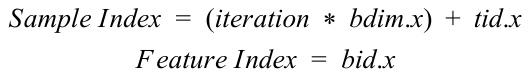
Here, iteration is the current kernel launch iteration. Launching the kernel in this manner allows us to have a simpler index computation, removing the need to perform a modulus and division for each thread. This also allows us to load the features into shared memory and reduce the number of global memory accesses for each thread. The downside is that now we must launch the kernel (N / block_size) times. Here is the parallel training kernel pseudo-code using shared memory:

Classification

The approach to classification on the GPU follows the same structure as the training implementation. Much like the sequential code, the main difference is the function byproducts. The classification kernel produces a results vector of the classification label and an errors vector for each feature. Here is the parallel classification kernel pseudo-code:

Again, we followed the same structure as the training kernel, in which we loaded the weights into constant memory and modified the kernel to load the features into shared memory and relaunch the kernel in iterations with new launch parameters. Here is the parallel classification kernel pseudo-code using shared memory:

IV. Results

The datasets used in this paper we sourced from the Extended Yale Face Database [6][7]. There are 4903 positive samples of aligned, cropped (168x192) face images included in this set. The images were then resized to reduce the shape of each image to 24x24 pixel images. Our negative sample dataset was sourced from Google’s Open Images Dataset V6 and manually scrubbed to remove any images including a face. The images were then resized to 48x48 pixel images and split into 4 subregions. These subregions are what we use as our negative samples. To test how our GPU implementations scale with the size of our dataset, we used several different levels of sample sizes and graphed the resulting computation time for each function.

Note: There is a current limit of 8,000 samples that can be used in the system due to current memory inefficiencies in the implementation.

Integral Images

Taking a look at the results for the integral images variants, we can see that the CPU version of this function is faster than all of the GPU kernels for computing integral images. This is due in part to the number of samples we could utilize in this implementation. It can not be stated with complete certainty that the CPU runtime will surpass our GPU implementation runtimes, however the data does trend in this direction. This would make sense for low sample numbers to cause the GPU code to take a longer time to execute as there is a lot more overhead involved. In order to compute the integral images of all samples in a dataset, we must launch four kernels. The first to scan through the rows of the images, the second to take the transpose, the third to scan through all the columns, and the fourth to take the transpose again and return the images to their proper orientation. As we observe, this overhead supersedes the benefits of the parallel execution for low sample sizes. We can also observe, as previously stated, the inefficiency of using pointer allocation on the device as opposed to pitched data allocation.

Training

The results for the training kernel proved to hold a much better execution time than the CPU counterpart. We observe that at very low sample sizes, the GPU and CPU versions were very similar in computation time; however, as the samples increased, the rate of increase in execution time for the CPU code was much faster than that of the GPU code. We did not have much of the overhead that was involved in the Integral Image kernels, so even with this low sample size of 8,000 images, we can see much better performances overall from the parallel executions. We also can observe the shared memory version of the kernel starts to overtake the original kernel implementation at higher sample sizes.

Classification

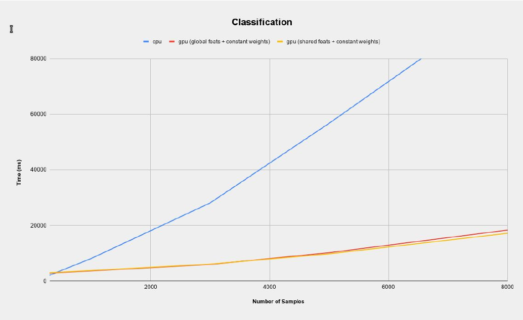
Since the classification kernel is essentially identical to that of the training kernel, we notice very similar results. The CPU and GPU implementations start with similar execution times at low samples, with the CPU version increasing at a much faster rate with an increase in sample size. We also notice the same pattern of the shared memory adaptation of the kernel showing slightly better execution times at larger sample sizes.

References

[1] Viola, P. & Jones, M. “Rapid object detection using a boosted cascade of simple features.” Proceedings of the 2001 IEEE Computer Society Conference on Computer Vision and Pattern Recognition. CVPR 2001 (2001).

[2] P. M. Kogge and H. S. Stone, “A parallel algorithm for the efficient solution of a general class of recurrence equations,” IEEE Transactions on Computers, vol. C-22, no. 8, pp. 786–793, 1973.

[3] Cen, P. “Study of Viola-Jones Real Time Face Detector.” Stanford University. 2016

[5] Jain, V. & Patel, D. A GPU Based Implementation of Robust Face Detection System. Procedia Computer Science 87, 156–163 (2016).

[6] Lee, Kuang-Chih, et al. “Acquiring Linear Subspaces for Face Recognition under Variable Lighting.” IEEE Transactions on Pattern Analysis and Machine Intelligence, vol. 27, no. 5, 2005, pp. 684–698., doi:10.1109/tpami.2005.92.

[7] Georghiades, A.s., et al. “From Few to Many: Illumination Cone Models for Face Recognition under Variable Lighting and Pose.” IEEE Transactions on Pattern Analysis and Machine Intelligence, vol. 23, no. 6, 2001, pp. 643–660., doi:10.1109/34.927464.